ODE Model VS DAE Model
Power system dynamics are evaluated either by the ordinary differential equation (ODE) form or by the differential-algebraic equation (DAE) form. In the DAE formulation, the algebraic part is usually derived from the decoupling of fast-slow dynamics, or some hard limits and algebraic relations from engineering designs. A DAE system is also called a constrained dynamical system whose dynamics are restricted on the manifold induced by the algebraic constraints. These algebraic constraints can substantially complicate the analysis of regions of attractions and stability boundaries. The following plot presents an illustrative comparison between an ODE system and a DAE system.
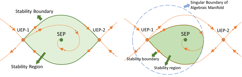
The left hand side of the above plot shows the stability region (light green shaded area) of an ODE system. The stability boundary comprises the stable manifolds of the corresponding type-1 unstable equilibrium points (UEPs). The right hand side plot shows the stability region (light green shaded area) of a DAE system. The stability boundary comprises a part of the stable manifold of a type-1 UEP, a part of the singular boundary induced by the algebraic constraint, and a part of a particular dynamical flow.
To evaluate the stability boundary of a power system dynamical model in the DAE form, the singular surface of the manifold induced by the algebraic constraints is of great importance.
Variations of Algebraic Manifold under Different Static Load Models
By continuously changing the static load model for a power system DAE system, the corresponding algebraic manifold can be altered substantially, which further changes the singular surface. Meanwhile, the number of equilibrium points and their types are also changed. A comprehensive study can be found in Influence of Load Models on Equilibria, Stability and Algebraic Manifolds of Power System Differential-Algebraic System. The following plots only present the variations of the algebraic manifold and the singular surfaces for a 9-bus test case.
The upper-left plot shows the equilirium points (black circles), algebraic manifold (purple surface) and the singular surface (blue curve) for the 9-bus case with constant power load model. The upper-middle plot shows the equilirium points, the algebraic manifold and the singular surfaces for the 9-bus case with 80% constant power load + 20% constant impedance load (the total load demand at the high-voltage solution is unchanged from the constant power load model). The upper-right plot shows the equilirium points, the algebraic manifold and the singular surfaces for the 9-bus case with 60% constant power load + 40% constant impedance load. The lower-left plot shows the equilirium points, the algebraic manifold and the singular surfaces for the 9-bus case with 40% constant power load + 60% constant impedance load. The lower-middle plot shows the equilirium points, the algebraic manifold and the singular surfaces for the 9-bus case with 20% constant power load + 80% constant impedance load. The lower-right plot shows the equilirium points, the algebraic manifold and the singular surfaces for the 9-bus case with 3% constant power load + 97% constant impedance load.
The plots show that the manifold becomes increasingly complicated with many folds as the load model continuously changes. More observations are discussed in the paper mentioned above.